Birds Astronomy Site: Processing Example

I have had several people ask me about the processing steps I use when creating a final planetary image so I thought it might be useful to put up a quick web page that does just that.

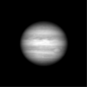
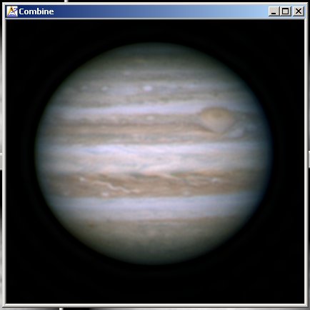
This is what we're going to create by the end of this example

Processing philosophy and Information Preservation

If we consider only the amount of information present in our raw frames as the starting point, then each step along the way of the processing pipeline can either preserve that information, or lose some of it. Once information is lost in one stage, there is no way to get it back in later stages. It's gone forever.

In general, most of the "enhancing" stages in image processing work by selectively discarding the information you have decided is not required in exchange for highlighting the information you think is important. However, there is still going to be less information in the resulting image than you start with, hopefully you chose wisely and discarded only information that wasn't going to be required in later stages!

What sort of information gets lost? I hear you ask...well, any operation that enhances edges, like wavelets, unsharp masking or deconvolution, is doing so at the expense of the subtle gradient changes in the image. An edge that might start out to have 64 shades from one side to the other (a blurry edge) might end up with only 16 shades after processing covering the same range of brightness, or maybe an even larger range! So the "information" contained in the original 64 shades has been compressed into only 16 shades and some of the original values must be lost.

Is Information loss really important?

My rule of thumb is to only use information-preserving stages early on, and then be very selective about the order of the later stages so that you only discard information that you no longer really need.

Like all things in image processing, this is a compromise. You can't help discard information, but it's very important that you recognise when it's happening, and adjust the severity of the later processing stages to compensate.

How can I measure the information loss?

One very important point... never store any of the intermediate results in an image format that loses information, or you'll find that the battle is already lost. e.g. JPEG format is usually very lossy, as you can easily see by looking at a JPEG image as compared to the original uncompressed version.

The Camera

Also, you can change your mind later about how you process images and try something different, but you can't change the raw data from the camera once you've captured it. This raw data is the starting point for all of your processing so it must preserve as much of the information that fell into your camera as possible!

My current astronomy camera is a Unibrain fire-i board camera (monochrome). This camera uses a 640x480 pixel sensor from Sony called ICX084BL that is quite sensitive. This sensor is the monochrome counterpart of the ICX084BQ colour sensor used in popular cameras such as the ToUCam.

This camera uses a high speed data connection to the host PC (firewire) that allows it to send the raw data exactly as it is received by the onboard sensor. I normally operate this camera in either 25 or 30 frames per second mode, so the amount of raw data being sent by the camera to the PC comes to:

	640 x 480 = 307200 pixels

	Each pixel is one byte (8 bits) of grey level, so...

	307200 X 25 = 7,680,000 bytes (7.3Mb) per second, at 25 fps.

I choose to store these frames in BMP format because it's simple, fast and information-preserving. A BMP file consists of a small header followed by the raw data. I can write that fast enough to sustain 7.3Mb/second throughput to my hard disk. (Actually, for bizarre reasons, frames written like this will be inverted because the BMP standard stores the image from last line -> first line, but I couldn't be bothered wasting CPU time fixing my raw images to be in that order. I store them in the order that the come out of the camera, i.e. first line -> last line).

No information is lost in this stage. I normally end up with about 3000 frames of monochrome data (1000 through a red filter, 1000 through a green filter and 1000 through a blue filter) stored in uncompressed format in BMP files on my hard disk. This comes to about 920Mb of data for a single imaging run.

Now I'm free to play around with different imaging techniques, confident that I'm starting with the maximum amount of information possible given my telescope setup.

RGB vs Colour Imaging

Let me quickly explain the difference, and why we can get away with imaging the colour separately...

A colour camera captures red, green and blue pixels simultaneously. The 640x480 pixels in its sensor are divided in groups, and each group is sensitive to one particular colour. The most popular format has half the pixels sensitive to green, 1/4 sensitive to red and 1/4 sensitive to blue. This arrangement is chosen to match with a popular format for compressed video called "4:2:2 YUV", and so the camera can easily convert this colour data into a colour video stream with little or no effort.

The problem for us astronomers is that these cameras are already discarding information, even before we can get it to the PC! Only 1/2 of the green data falling into the camera is captured, and only 1/4 of the red and blue data is captured. As a result of this "compromise" only about one third of the light falling into the camera is actually recorded. Each pixel only records one of the three colour components that strike it.

Now many people will ltell you that this is quite ok, because the human eye is not very sensitive to red and blue so it's no big deal that this information is lost at the camera. My counterpoint is that we do need all the information since we'll be adding together many frames to create a single result - a very different scenario to live video where each frame is displayed and then discarded. It may certainly be true that the human eye will have trouble seeing red/blue detail in a live video stream, but when all those frames are captured and processed to create a static image, chrominance (red/blue) problems become much easier to see. Artifacts caused by the lower information content have been exaggerated by later processing stages and become quite visible.

A monochrome camera captures all pixels equally, so a monochrome camera + colour filters allows for full resolution imaging in red,green and blue - but not all at the same time of course. This is where we have a slice of luck, since planets are relatively slow changing objects we can image these three colours seperately and then combine them later to make a colour image.

Not all planets change at the same rate, and in fact Jupiter is the most demanding target because of its high rotational speed. It turns one degree on 90 seconds - not very long to finish an imaging run! It is this property that sets an upper limit on separate RGB imaging, if you take too long then the final set of frames (blue, say) will no longer line up with the initial (red) frames, and so a temporal distortion is introduced, leading to another type of information loss (features that were visible near the limb in the early frames are no longer visible in the latter frames).

With my firewire camera and a shutter speed of 33ms (30 fps), I can record 1000 frames in about 30 seconds. So the full imaging run of red,green,blue takes about 90 seconds. This is the upper limit that I have imposed to minimise this image skew caused by rotation.

A colour firewire camera operating at 30fps over this same period would record less spacial resolution but (because each colour is recorded for 90 seconds instead of 30) may well have a better signal-to-noise ratio. In practice however, colour cameras like the ToUCam will only record at 10fps, or 5fps, so the amount of raw data collected is much lower than the firewire camera and so the increased s/n that is theoretically possible is not realised. This means that the ToUCam will have lower resolution and lower s/n. This has to be offset against the convenience of capturing all three colour channels simultaneously.

Some real data

To make this data available to those of you with slower connections, I have made two versions of each data file:

* The BMP version contains uncompressed BMP format frames at full resolution and quality, but each archive
  is approximately 27Mb in size.

* The JPG version contains high quality JPEG frames, but it is significantly smaller (12Mb). The final result will
  be a little worse if you use the JPEG version, but the difference in practice may not be noticeable.

• 20050417-1456 RED (BMP) (RED archive, approx 27Mb)
• 20050417-1456 GRN (BMP) (GREEN archive, approx 27Mb)
• 20050417-1456 BLU (BMP) (BLUE archive, approx 27Mb)

OR

• 20050417-1456 RED (JPG) (RED archive, approx 12Mb)
• 20050417-1456 GRN (JPG) (GREEN archive, approx 12Mb)
• 20050417-1456 BLU (JPG) (BLUE archive, approx 12Mb)

If you want to follow along and process this raw data yourself, please take the time to download the three archives listed here and unpack them. You should end up with 3000 image files arranged in folders called R, G and B.

You will see that each of these frames is 400x400 pixels in size. I have slightly pre-processed these frames to save a bit of space by centering the planet in each frame and cropping down from the original (640x480) size to 400x400. This makes the frames a lot faster to process since they are only half the size of the originals, but again no information has been discarded since the planet only takes up the middle part of each frame.

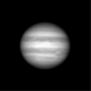
For those of you who just want to read but not work through this example, here is one of each of these raw frames so you can see what they look like:

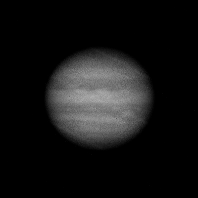Sample RED Frame

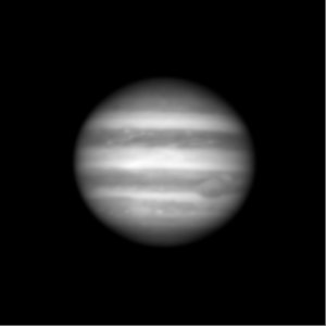
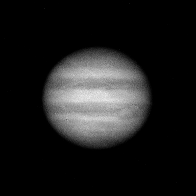Sample GREEN Frame

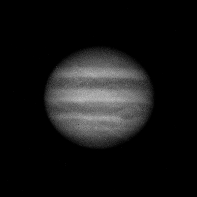Sample BLUE Frame

The program I used to centre the planet and crop the frames is called ppmcentre, and is available here. (Note: You don't need this program for the tutorial, but if you choose to capture raw data in the same way that I do then you might like to try using it to pre-process the images before you load them into registax).

Processing Stage 1: Registax

The goal for this stage is to stack together the red frames to make a single image, then repeat for the green and blue frames. We will end up with three "stacked" images at the end.

Here are the steps to follow:

• Start Registax
• In Windows Explorer, select all the red frames (highlight the R directory, press Control-A).
• Drap-drop all those frames onto Registax. You will see the frame counter near the bottom indicate 1000 frames.
• Click on the Framelist tab at the right side, and select "sort". Now the frames are in order from 00000 through 01000.
• Set the Alignment Box size (top) to 128.
• select the Gradient quality estimator.
• Click near the centre of the frame that's displayed. You should see a white box that almost covers the entire centre region of the planet.
• A new window called "FFT Spectrum" will be displayed. Change the value of the FFT filter to 2 (it will probably start out at a high value like 80, a very poor guess indeed!). When you do this you will see the graphical display in the FFT filter window change to have large areas of red/yellow/green. This is good, since it means that large parts of our image data will be used for alignment.

  NOTE: If you have poor quality data, then this FFT filter should be set a bit larger. In general, you should set it to the smallest feature size that you think is present in your image but larger than the size of noise. By setting it to 2 I am asking it to use features that are 2 pixels or larger in my image for alignment purposes and ignore features that are smaller than that size (e.g. noise will typically be 1 pixel in size so it will be filtered out).

• Click Align and watch while the alignment run happens. This pass does two things, it calculates the sharpness of each frame (i.e. how much information each frame contains) and also calculates an alignment difference between each frame and the first frame.
• Click Limit after this pass has finished.

  At the end of this first pass, the frames are sorted from sharpest -> softest, using the Gradient algorithm. If it's worked then you should see frame 00778 displayed as the first frame. This is the sharpest red frame in the set.

• Now we do the align stage again. This time we will be using frame 00778 as our reference frame as it has been selected as the best. Click on the Align tab to switch back to the Alignment page, then click in the middle of the displayed frame to set the alignment region - this should be frame 00778. Once again the FFT will be displayed with an incorrect filter size, change it back to 2 and hit Align.
• When it's finished, move the frame slider at the bottom of the screen to the left until it says "700/1001" and click on Limit. This sets registax to only process the best 700 frames.
• We will be resampling the raw frames to a larger size for the next stages, so tick the Resampling box, set the resampling algorithm to Mitchell and the Factor to 1.5.
• The next step is to create a reference frame. You will see an area at the top of the screen labelled Reference Frame. Set the number of frames to 50 and click Create. Registax will do a quick alignment & stack of the first 50 frames in the list, i.e. the best 50 frames.
• Click OK to dismiss the dialog box that appears when this is finished. Now we must enhance this stacked image so that it is suitable to use as a reference frame for the rest of the processing. In the wavelets section, set layer 3 to 5.8. This gives an enhanced image that is still relatively close in detail to the raw frames but with much less noise. Click Continue.
• Once again, dismiss the dialog window that comes up. Then click on Optimize to start the alignment process. This will align all of the frames against the reference frame created in the previous step. You should see the frame alignment (blue line) drop down close to the bottom of the graph for each frame that's processed. It normally takes 3 passes for me before this stage is finished.
• Switch to the Stack page. Make sure that Histo-Stretch is ticked on. Click Stack and wait while the 700 frames are stacked.
• When the stacking is done, change to the Wavelets page and click Reset to get rid of the settings from the earlier (create reference frame) stage. Now click on Save Image in the top right corner of the screen and save this image as "r.fit", setting the file type to FITS (16 Bit).

• That is the end of processing for the Red data. Switch back to the Align page, open the framelist and click "Empty List".
• Using Windows Explorer, select all the Green frames, and drag-drop them into registax. Now follow this procedure through again for these green frames, and save the result as "g.fit".
• Repeat for the Blue frames, saving the result as "b.fit".

In the end, you will have three 16-bit FITS files that look like this:

Red FITS image Download r.fit (700kb)

Green FITS image Download g.fit (700kb)

Blue FITS image Download b.fit (700kb)

Have we lost information in this stage? Yes, rather a lot of it. With luck we have thrown away mostly noise and not too much important data, but it's not possible to easily separate the two so some data will be lost. Hopefully not too much.

Fixing the FITS files

I have written a small program called fixfits that will fix these files and make them compatible with the other programs that we will be using in this tutorial. You can download it from my software page and run it from a command prompt with the command:

	fixfits.exe *.fit

Processing Stage 2: Deconvolution and Merging in Astra Image

You can get this package from www.phasespace.com.au

The goal of this stage is to load each of these FIT files into Astra Image, deconvolute them, filter and then recombine them to form a colour image.

Here is what we will do in Astra Image:

• Start Astra Image, and open the file r.fit.
• Use the mouse to select a region that surrounds the planet image, leaving plenty of space around it. As a guide, the edges of the selection box should be about halfway between the edge of the planet and the outside edge of the image. If in doubt, look at the images below to see how much space I have left after cropping.
• Click on the Crop icon (or via the menus, selet process -> Crop. In the dialog box that comes up select Get from ROI. This will set the crop dimensions to the region that you selected with the mouse.
• Click OK and a new window will appear showing the cropped area.
• Close the original window, keeping the new, smaller window. The new image is automatically named after the process that created it, so it's called "crop".
• make sure the "crop" window is selected (it should be, its the only window) and click on the LR icon in the toolbar. This brings up the Lucy Richardson deconvolution dialog. Set Iterations to 40, make sure PSF Type is set to Gaussian and Curve Radius is set to 2, then Click OK. After a while a new image will appear showing the deconvoluted image. Compare it to the original image - you should find that more structure is visible in the deconvoluted image than previously.

  This step throws away some information in the original image in the process of attempting to reverse the blurring process. You can find a lot more information on this algorithm (Richardson-Lucy) on the net.

• With this new image selected, open the "Filter -> FFT Filter" dialog. Set the filter type to Ideal Highpass and the Filter Strength to 16, other values left on their defaults. Click OK and a new image window is displayed showing the result of applying this filter to the LR image. Once again you should find that more structure is visible in this image, again at the expense of discarding some other information from the source image.
• Set the Image Title on this final image to "r" (Edit -> Image Title).

• Now we want to repeat these steps on the green and blue images. One important point to notice: Astra Image will remember the parameters that you used previously, and we want to keep those unchanged. So, when you crop the green image DO NOT change the values in the dialog, just press OK. This ensures that each of these cropped images will corretly align when we recombine them.

Here's what these images should look like:

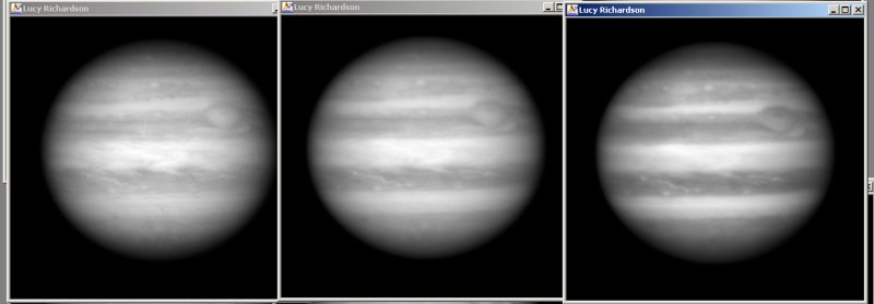
The three (red, green, blue) images after cropping and RL deconvolution. Notice that more structure is becoming visible in these images.

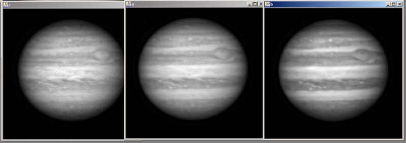
The three (red,green,blue) images after cropping, RL deconvolution and FFT filtering. More detail again is visible.

Recombining to make a colour image

• Click on the RGB Combine icon (or via the menus, Process -> RGB Combine). A dialog box will appear that has already selected your r , g, b images - you did remember to rename the FFT produced images didn't you? They should be named "r", "g" and "b" so this combiner wil automatically select them.
• Press the Update button, and you will see in the preview window how the combined image will look. The first thing you'll notice when you scroll around and look at this preview image is that the three colours don't line up. This is caused by a number of things, remember that the red frames were captured about 60 seconds earlier then the blue frames, and so the planet has rotated a bit between them. Also the registax alignment pass may have moved each colour plane a little, etc. It doesn't matter, cause this dialog box has RGB offset controls that we will use to realign the colour planes.
• Zoom in two steps, making the preview image much larger, and the colour alignment errors much more obvious.
• Now we must tinker with the offset values to see if we can align these colour planes properly. It helps a lot if you can locate a part of the image that's supposed to be white. In this case there is a prominent white spot near the upper centre of Jupiters image - it shows up clearly on all three images. While zoomed in, move the preview window so that area is visible.
• Initially you'll see that the red,green and blue images are misaligned. What you must do now is make small changes to the X and Y offsets for each colour plane, pressing the Update button after each change, until you can get those regions to line up as best you can.
• When that's done, zoom back out to the original scale to check out the result. With any luck it now looks a lot more like Jupiter should!
• Finally, we have to adjust the colour balance of each colour plane. This is necessary due to a quirk of the FITS file format that we have been using to store the stacked data. Each colour plane was automatically adjusted to have its brightness evenly spread across the range black -> bright (that's what the histo-stretch in Registax did), so now that we have recombined these planes it's necessary to re-adjust their brightness.
• To see what the current image looks like, just click OK and the recombined window will appear. It looks too green so we have to change the RGB combine colour weights to remove some green.
• Close the greenish jupiter window and click on the RGB Combine again. You'll see that it has remembered all the parameters, so just hit Update and it will re-create the image in the preview window.
• Change the Colour weighting for green from 1 to 1.1. It may seem counterintuitive, but making the colour weight larger actually decreases the weight of that colour. Click on Update to see what effect this has had. Now the image it too red. Set the Red colour weight to 1.05 and click Update again. Now it looks ok, so press OK to do the combine.

Let's take a moment to see some screenshots of these steps again:

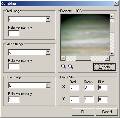	The RGB combining page when the images are first loaded. Notice that the red, green and blue planes don't align properly.
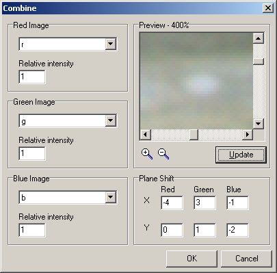
	We've zoomed in by 2 steps on a white oval storm near the top of Jupiters disk. This is a good guide to assist in calculating the correct colour plane offsets.
	After some trial and error, this is a good set of offsets.
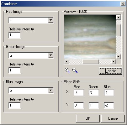	When we zoom out to the original size we can see that the colour planes now line up properly. The only remaining issue is to find the correct colour balance. Left like this the image will be much too green, this imbalance caused by my camera which is more sensitive to green light than red or blue and hence has produced a brigher image in green than the other colours. You can see this if you refer to the earlier raw images.
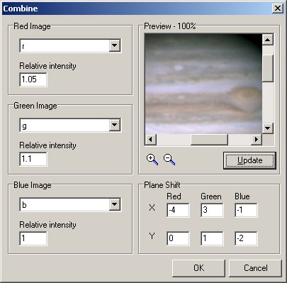	After some more trial and error I settle on Relative Intensities of 1.05, 1.1 and 1.0 for red,green and blue.
	After we hit OK then this is the combined image.

Now this is almost where we might choose to stop processing. Certainly the final image here is quite good and shows a wealth of detail. However there are a couple more steps we might take to bring out more detail still, at the expense of discarding yet more information from the image. Since we are right at the end of the processing pipeline, and there are no more stages to follow, we can be a bit more rutheless.

With the colour image selected, choose Filter -> Unsharp Mask, set the Blurring Strength size to Maximum and th Power to 1.5. Press OK and a new, sharper image is produced.

With this new image selected, choose Process -> Resample and set the width of the new image to 300. This represents almost a 1.5x reduction in size, undoing the 1.5x resample that was applied earlier in Registax. When you apply this change a smaller, sharper image is again produced, that looks like this:

Finale

Before you jump on the email to tell me that I'm doing this all wrong, and that you have a better system, please remember that I'm always changing my steps as a matter of course, trying to always find improvements. What I have documented here is just one way of going from raw data to a finished image, but I know that there are many other paths possible, and indeed I find myself almost always varying from this process (sometimes a little bit, sometimes a lot) here and there to search for improvements.

E.g. I will try adding a wavelets processing step somewhere, or change the order of some steps, maybe add a gamma-adjust step, etc. If I go wrong, then it's a simple matter of deleting the result and trying again.

One obvious change would be to include wavelet processing - either in registax, PixInsight, or other package. I used to use wavelets in registax as a matter of course but I have found that they discard a lot of information, and as a result I was limited in how much I could continue to process the images in later stages without severe artifacts showing up.

But it's all a balancing act. There are a lot of different ways to extract the visible data from these images, and I hope that this example has shown you something useful.

If you download the raw data for this example and find a different system that gives better results, please send me the details! If you write it up then I'll add a link from this page to your system so people can see how you do it, and what results you get.

And, of course, if your system's better than mine then I'll start using yours :-)

Anthony Wesley